TLDR 너무 길어서 안읽어
범주형 데이터 -> numeric : 인코딩
연속형 데이터 -> 범주형 데이터 : Binning
정답이 있는 답과 정답이 없는 답
통계학이 무엇인가요 ? _____________입니다. 하지만 제 생각에는 이런이런 부분도 고려해서 이런 것 이라고 생각합니다.
# Machine Learning 알고리즘 활용
(1) 직접 프로그래밍 수행
- Python + 패키지
-> statsmodels : https://www.statsmodels.org/
-> scikit-learn : https://scikit-learn.org
-> tensorflow : https://www.tensorflow.org
-> keras : https://keras.io
** Keras comes packaged with TensorFlow 2.0 as tensorflow.keras.
To start using Keras, simply install TensorFlow 2.0.
** Software suites containing a variety of machine learning algorithms
https://en.wikipedia.org/wiki/Machine_learning#Software
-> flask : https://flask.palletsprojects.com/en/1.1.x/
- R + 패키지
- Java + 패키지
- ...
(2) 비쥬얼 툴 활용
- RapidMiner : https://rapidminer.com/
- Tableau : https://www.tableau.com/ko-kr
- Weka : https://www.cs.waikato.ac.nz/ml/weka/
- Orange : http://orange.biolab.si
- Disco : https://fluxicon.com/disco
- Rattle : https://rattle.togaware.com/, http://me2.do/x5jliubo
- ...
(3) 제공되는 서비스 활용
- Google : https://cloud.google.com/ai-platform
- Microsoft : https://azure.microsoft.com/ko-kr/services/machine-learning/
- Amazon : https://aws.amazon.com/ko/machine-learning/
- IBM : https://www.ibm.com/watson/
- 네이버 : https://www.ncloud.com/
- ...
Scikit-learn
시킷 학습 | 소개 파이썬 데이터 과학 핸드북 (jakevdp.github.io)
import matplotlib.pyplot as plt
import numpy as np

rng = np.random.RandomState(42)
x = 10 * rng.rand(50)
y = 2 * x - 1 + rng.randn(50)
plt.scatter(x, y);

# 선형 회귀 모델 존재
from sklearn.linear_model import LinearRegression


# 2. 모델 하이퍼파라미터 선택
model = LinearRegression(fit_intercept=True)
model

# 3. 피쳐 매트릭스 및 대상 벡터로 데이터를 정렬
X = x[:, np.newaxis]
X.shape

# 4. 모델에 맞게 데이터에 맞게
model.fit(X, y)
model.coef_       # 데이터 정의와 비교하여 2의 입력 기울기와 매우 가깝다.
model.intercept_  # -1의 가로채기가 매우 심하다.


# 5. 알 수 없는 데이터에 대한 레이블 예측
xfit = np.linspace(-1, 11)

Xfit = xfit[:, np.newaxis]
yfit = model.predict(Xfit)
나이브베이즈
# Naive Bayes 분석
plt.scatter(x, y)
plt.plot(xfit, yfit);

from sklearn.cross_validation import train_test_split
Xtrain, Xtest, ytrain, ytest = train_test_split(X_iris, y_iris,
                                                random_state=1)
감독되지 않은 학습 예: 아이리스 치수
4차원으로 되어있는 아이리스 데이터를 2차원으로 차수를 감소시키는 것 : 주성분분석(PCA)
from sklearn.decomposition import PCA  # 1. Choose the model class
model = PCA(n_components=2)            # 2. Instantiate the model with hyperparameters
model.fit(X_iris)                      # 3. Fit to data. Notice y is not specified!
X_2D = model.transform(X_iris)         # 4. Transform the data to two dimensions
Seaborn으로 표시
iris['PCA1'] = X_2D[:, 0]
iris['PCA2'] = X_2D[:, 1]
sns.lmplot("PCA1", "PCA2", hue='species', data=iris, fit_reg=False);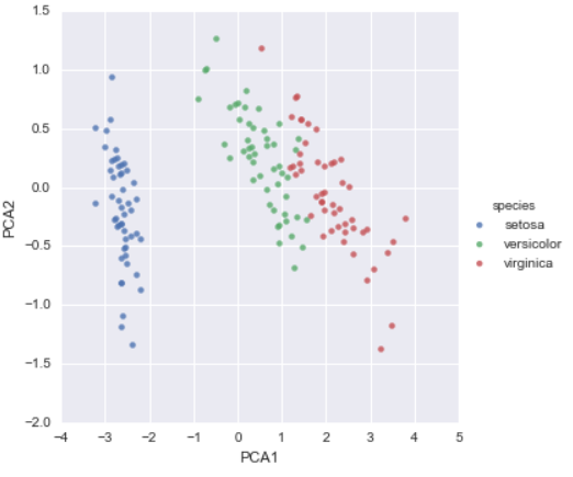
가우시안 혼합물 모델 (GMM)
from sklearn.mixture import GMM      # 1. Choose the model class
model = GMM(n_components=3,
            covariance_type='full')  # 2. Instantiate the model with hyperparameters
model.fit(X_iris)                    # 3. Fit to data. Notice y is not specified!
y_gmm = model.predict(X_iris)        # 4. Determine cluster labels
# Seaborn으로 플랏 표시
iris['cluster'] = y_gmm
sns.lmplot("PCA1", "PCA2", data=iris, hue='species',
col='cluster', fit_reg=False);
# setosa 종은 클러스터 0 내에서 완벽하게 분리되며,
# versicolor와 virginica 사이에 약간의 혼합이 남아있다.
# 현장에서 전문가들이 관찰하는 샘플 간의 관계에 대한 단서를 제공할 수 있다.
응용 프로그램: 손으로 쓴 숫자 탐색
숫자 데이터 로드 및 시각화
from sklearn.datasets import load_digits
digits = load_digits()
digits.images.shape
이미지 데이터는 3차원 배열입니다: 각각 8× 8개의 픽셀 그리드로 구성된 1,797개의 샘플. 이 중 처음 백 을 시각화해 봅시다.
import matplotlib.pyplot as plt

fig, axes = plt.subplots(10, 10, figsize=(8, 8),
                         subplot_kw={'xticks':[], 'yticks':[]},
                         gridspec_kw=dict(hspace=0.1, wspace=0.1))

for i, ax in enumerate(axes.flat):
    ax.imshow(digits.images[i], cmap='binary', interpolation='nearest')
    ax.text(0.05, 0.05, str(digits.target[i]),
            transform=ax.transAxes, color='green')
X = digits.data
X.shape
y = digits.target
y.shape # 1,797개의 샘플과 64개의 기능이 있음감독되지 않은 학습: 치수 감소
64차원에서 시각화를 하기엔 비효율적이기 때문에 차수를 2로 줄임. (Isomap 사용)
from sklearn.manifold import Isomap
iso = Isomap(n_components=2)
iso.fit(digits.data)
data_projected = iso.transform(digits.data)
data_projected.shape
plt.scatter(data_projected[:, 0], data_projected[:, 1], c=digits.target,
edgecolor='none', alpha=0.5,
cmap=plt.cm.get_cmap('spectral', 10))
plt.colorbar(label='digit label', ticks=range(10))
plt.clim(-0.5, 9.5);
숫자분류
# 가우시안 나이브 베이즈
Xtrain, Xtest, ytrain, ytest = train_test_split(X, y, random_state=0)

from sklearn.naive_bayes import GaussianNB
model = GaussianNB()
model.fit(Xtrain, ytrain)
y_model = model.predict(Xtest)

from sklearn.metrics import accuracy_score
accuracy_score(ytest, y_model)

from sklearn.metrics import confusion_matrix

mat = confusion_matrix(ytest, y_model)

sns.heatmap(mat, square=True, annot=True, cbar=False)
plt.xlabel('predicted value')
plt.ylabel('true value');
fig, axes = plt.subplots(10, 10, figsize=(8, 8),
                         subplot_kw={'xticks':[], 'yticks':[]},
                         gridspec_kw=dict(hspace=0.1, wspace=0.1))

test_images = Xtest.reshape(-1, 8, 8)

for i, ax in enumerate(axes.flat):
    ax.imshow(test_images[i], cmap='binary', interpolation='nearest')
    ax.text(0.05, 0.05, str(y_model[i]),
            transform=ax.transAxes,
            color='green' if (ytest[i] == y_model[i]) else 'red')
'인공지능 > 머신러닝' 카테고리의 다른 글
| 사이킷런으로 수행하는 타이타닉 생존자 예측 (0) | 2021.07.08 |
|---|---|
| sklearn.model (0) | 2021.07.08 |
| Sclkit - Learn을 이용 군집 (0) | 2021.07.07 |
| 툴 사용법 ( 이클립스, 주피터, 코랩, 아톰 ) (0) | 2021.07.06 |
| Scikit-Learn을 이용 회귀 (0) | 2021.07.06 |
